
Part III.
Introduction
To understand the effects of a strategic rebalancing schedule, I began a study that compares multiple rebalancing strategies. The premise is that people cannot decide when to sell, and systematic methods to buy and sell would take emotions out of the equation and might work better. I choose to start with a long-only portfolio that consists of investments in funds which are representative of an array of global asset classes. I identify each accordingly as
Market Conditions
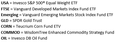
First, I look to describe the general performance of the components of the portfolio across this timeline.
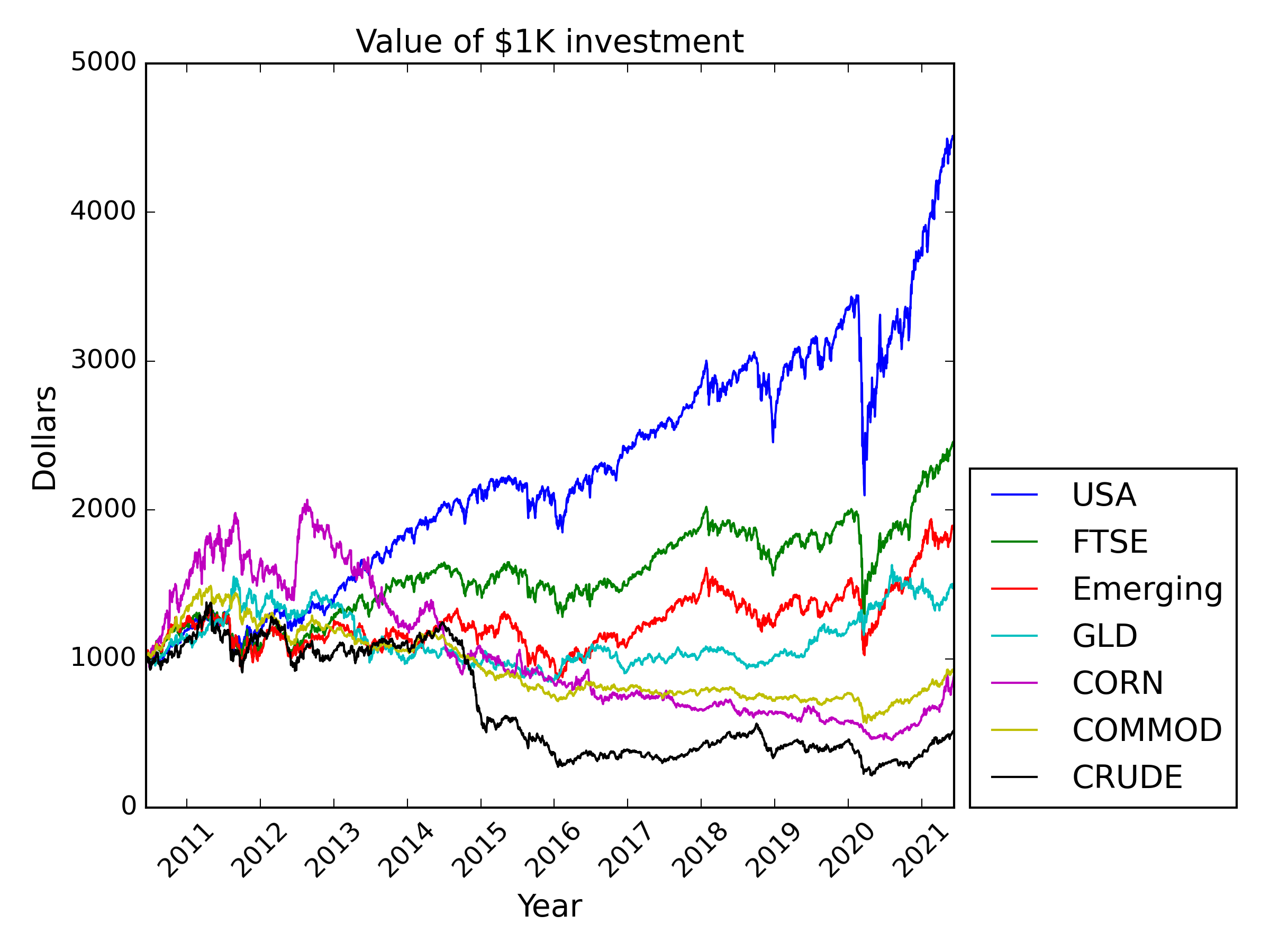
The US stock market was a bull in this decade. Others not so much. There were a few times of higher volatility, notably around Aug 8, 2011, Jun 24, 2016, and Mar 9, 2020. These are indicated in the noise plot below
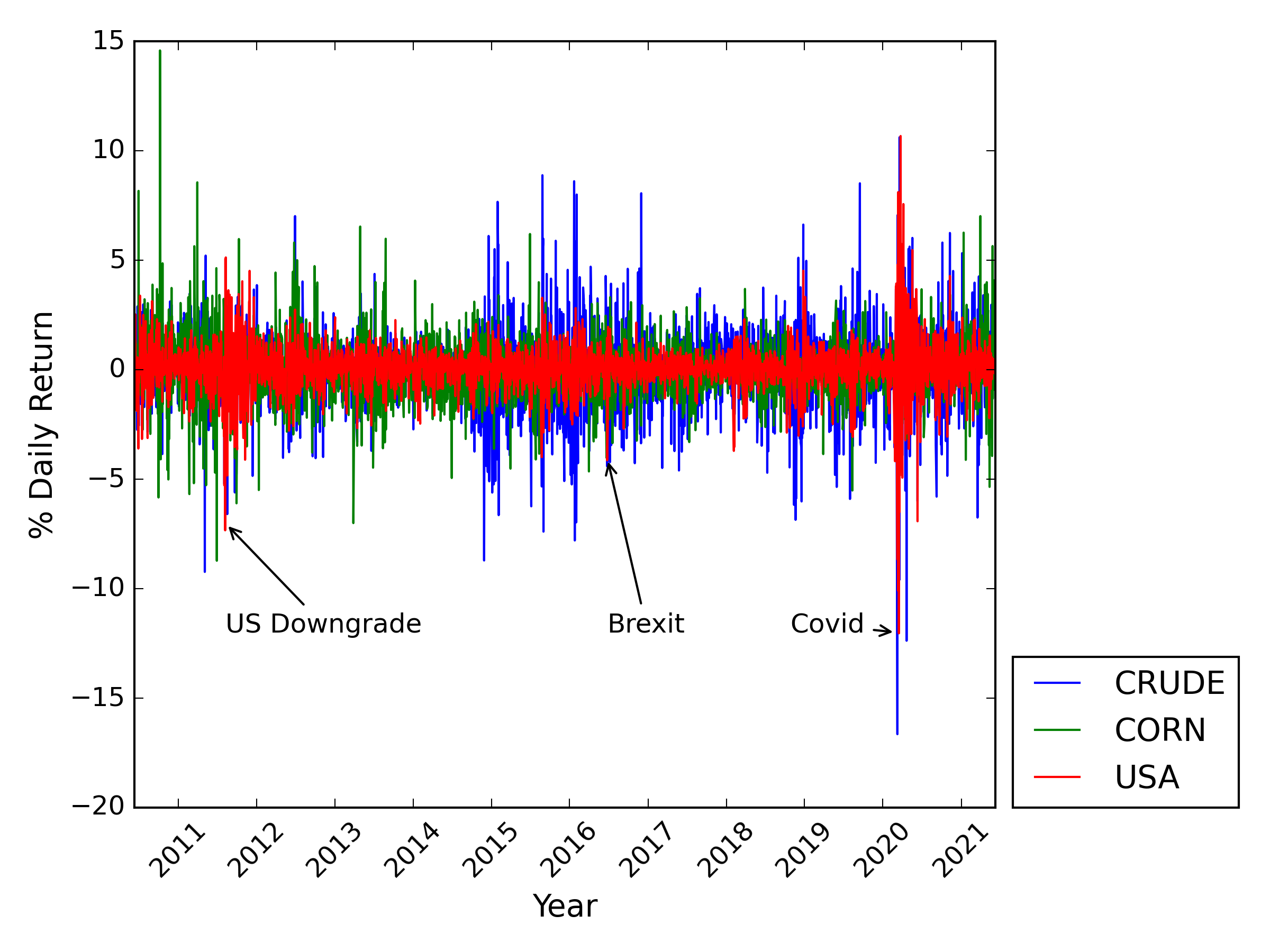
The most negative return of the dataset occurred in Crude Oil prices in 2020, and the most positive return occurred in Corn prices in 2010. Looking for outliers from another point of view,
one can qualitatively observe that the extreme days are mostly offset by opposite sign days of similar magnitude.
Buy and Hold strategy, US stocks only
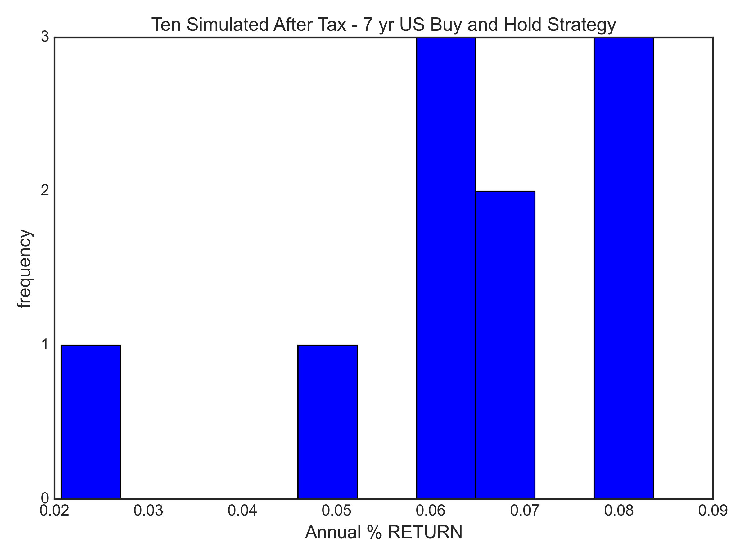
As a baseline, I ran simulations for a buy and hold strategy. Each simulation starts with the initial target diversification and is allowed to stray from the target weighting without any rebalancing. I simulated multiple 7-year holding periods, each with different start dates. I adjust the results for each simulation for the resulting capital-gains taxes that would affect after-tax return.
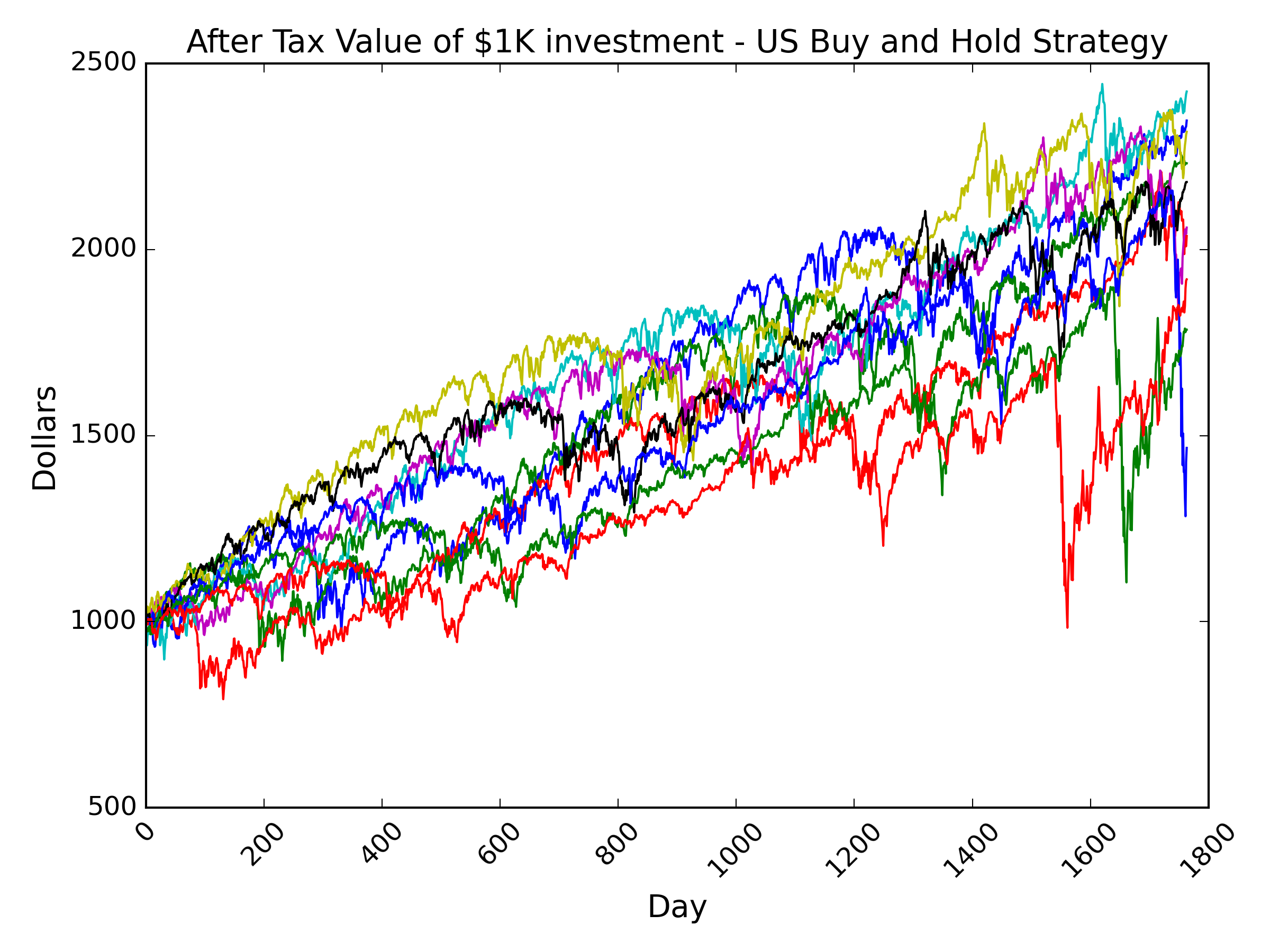
These US equal weighted stock ETF returns were bullish regardless of starting date, within the 2010-2021 period. Annualized after tax returns of the above simulations are displayed below.
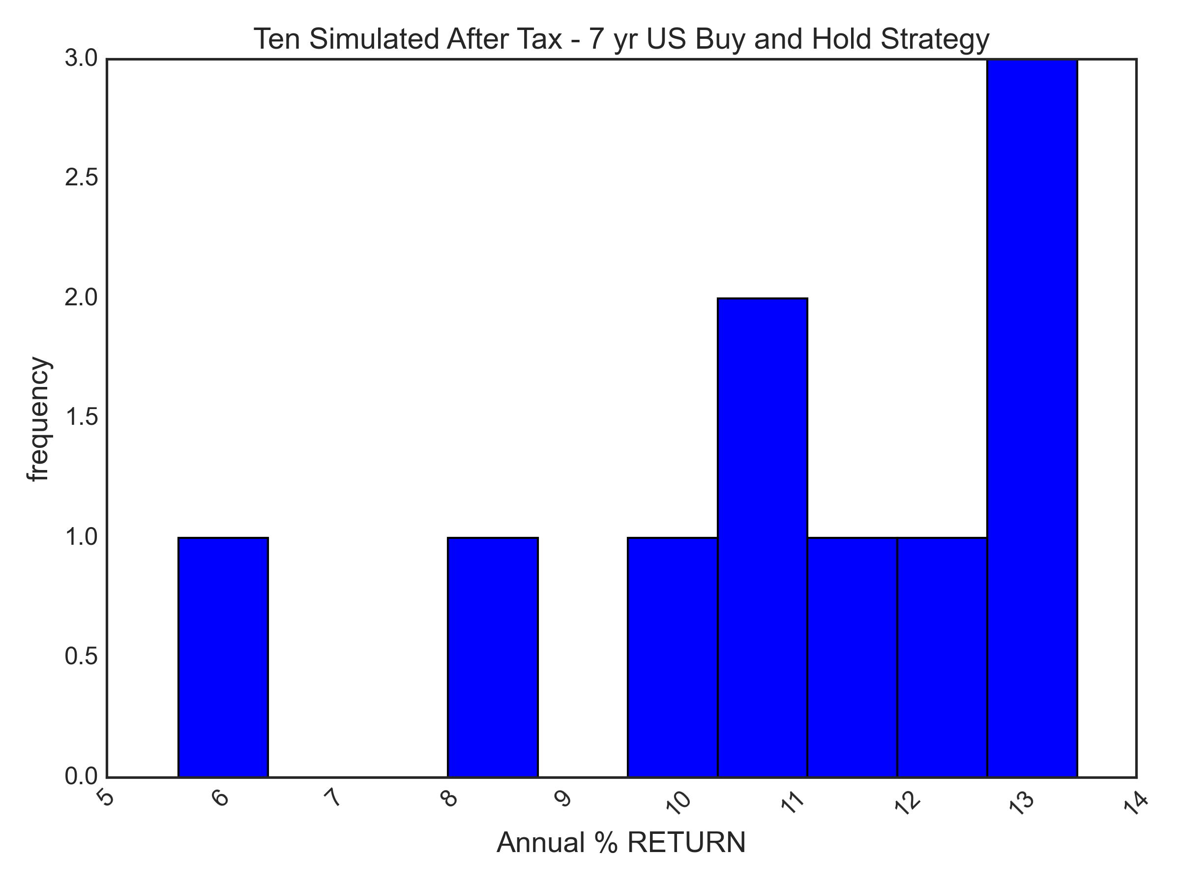
The median return of the 10 simulations is 11.3%. However, this is the US only portfolio, and I still need to describe the globally diversified portfolio.
Global Portfolio, Buy and Hold
To completely establish the Buy and Hold strategy baseline, I create a portfolio with the stated target diversification across the global asset classes.
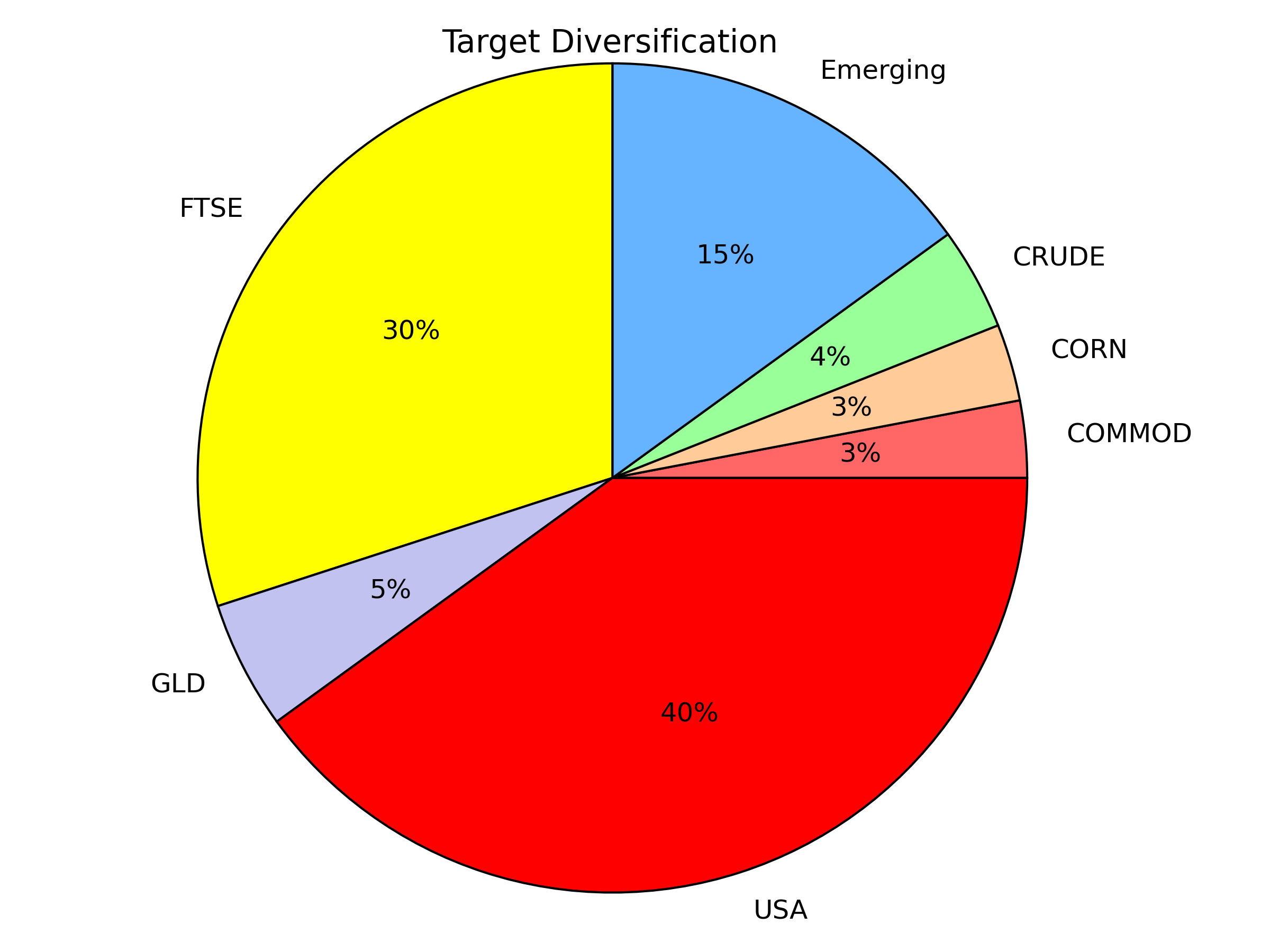
A risk taker’s diversification.
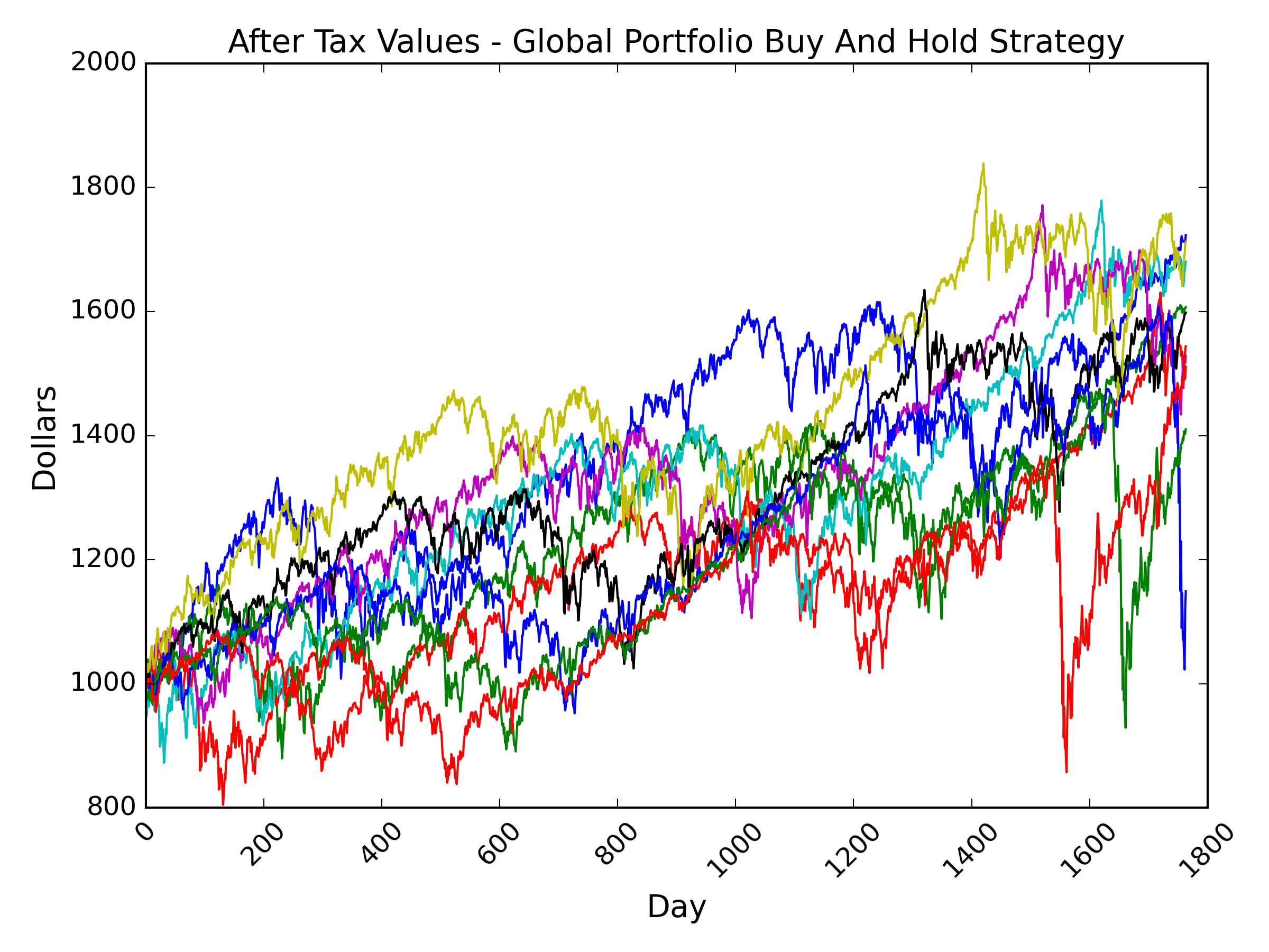 The median annualized return for the global buy and hold portfolio is 6.6%.
During this 2010-2021 period, the globalization of the portfolio reduced the expected return compared to a US only portfolio. I now seek to clarify if the global portfolio indeed was riskier than the US only one in terms of risk-adjusted returns. To do this, I can visually compare, or can calculate Sharpe Ratios.
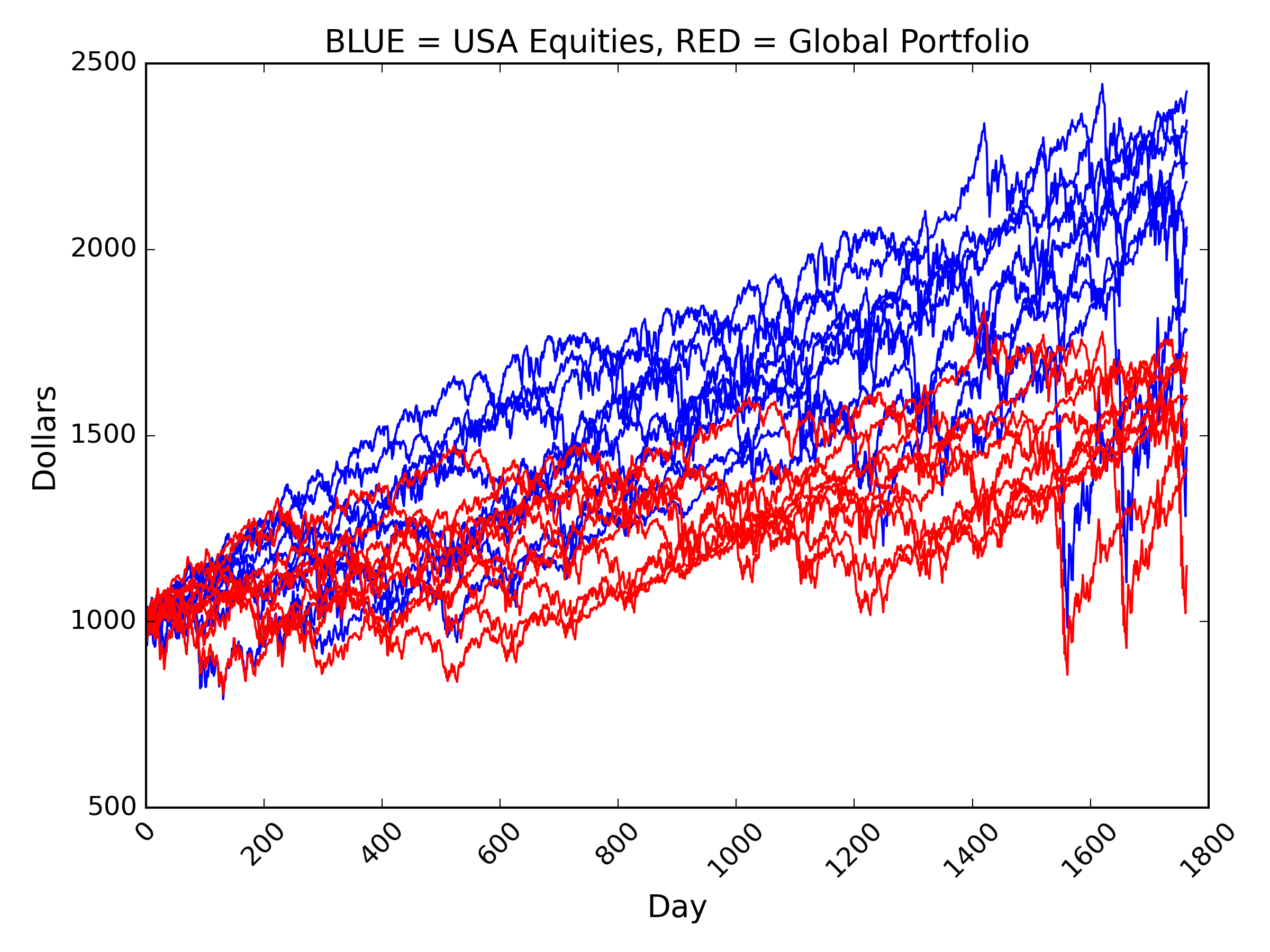
Visually speaking, the red grouping in the above is the global portfolio, and to the eye it’s variance looks slightly less than the America only portfolio. However, this does not mean it is less risky per unit of return received, in other words, in terms of the Sharpe Ratio. In comparing the ratios, In comparing the ratios,
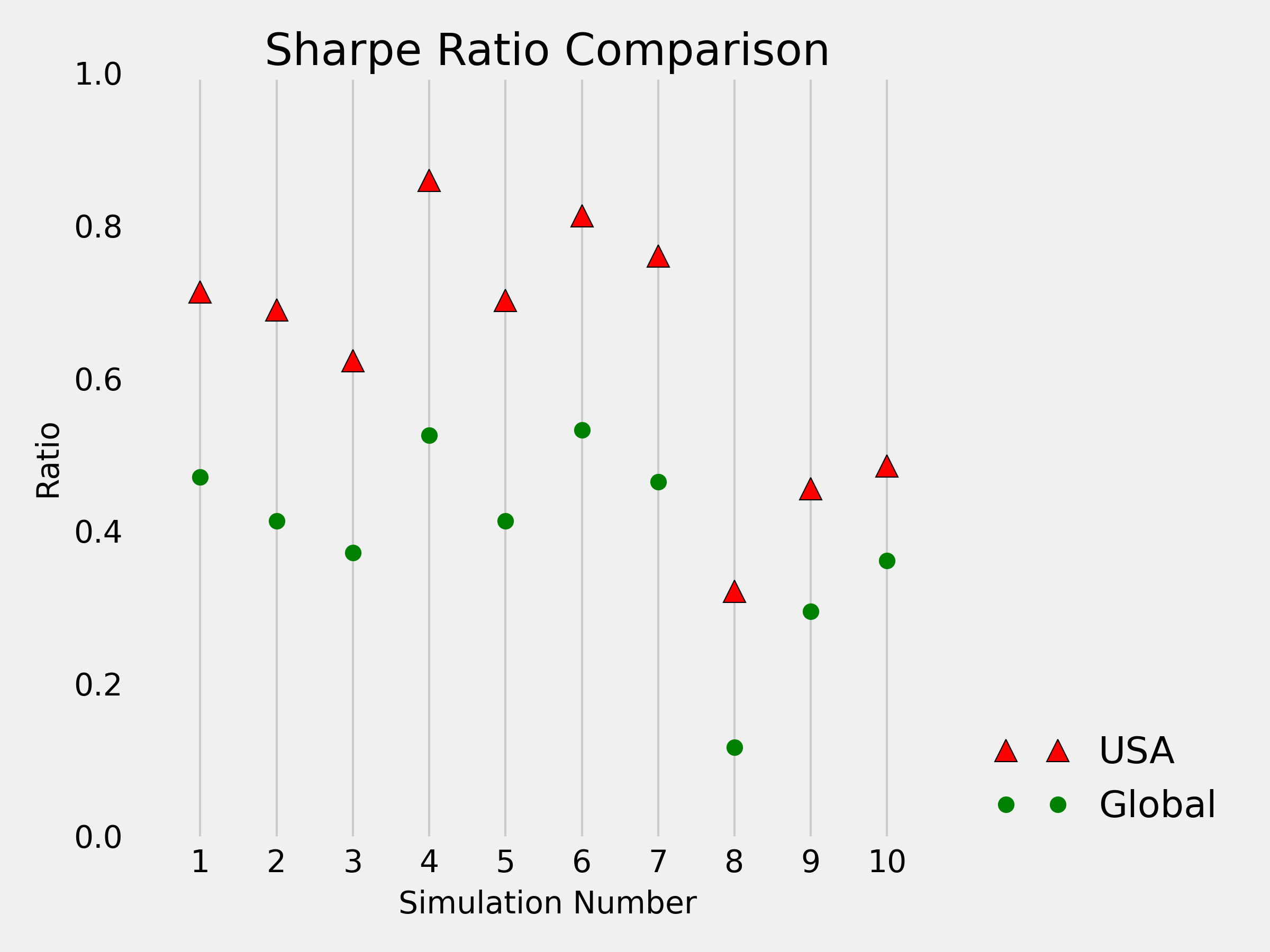
although the variance of returns in the global period was visually lower in the global portfolio, the relative Sharpe Ratios confirm that the global portfolio was risker on a risk-adjusted basis. Sharpe Ratios indicate the amount of return per unit of risk, and a higher relative Sharpe ratio indicates lower risk.
A less attractive riskiness in globalizing is the case for the buy and hold strategy. Perhaps it is would not be the case if we performed periodic rebalancing to the target portfolio distribution, which I intend to look at in the future.
Conclusion
Here I have compared buy and hold portfolios within 2010 – 2021. Moreover, I set the foundation for determining whether a less emotional and perhaps more rational trading strategy may help. I start with buy and hold strategies because they are what investors might do if they are caught like a deer in the headlights and then go like an ostrich with their head in the sand. This investor never sells, because he or she can’t decide to, or assumes the investment is bound to come back as soon as they sell.
Strategies of periodic rebalancing have been claimed to improve returns (Galen Burghardt, Managed Futures for Institutional Investors). However, this is not clear to be true regardless of timeframe. Increased turnover implies increased taxation. So, at what distance of horizon can we expect taxation to overwhelm the benefits?
![]()
![]()
![]()