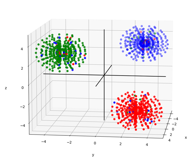
To test the behavior of an algorithm and determine if it works properly, I created a test set with 3 dimensions and 3 classifications from distributions that are defined. In this case they are represented by 3 separate spheres in different quadrants of space.
I generated 5% errors into the test set. For example, the green sphere has 5 percent red and blue points in it. In the spirit of the test, I expect a good model will have roughly 5% error in prediction.

Figure 1. The dataset in question with 5% problematic points.
CART (Classification and Regression Tree) algorithm
Before tackling this dataset, I backtrack and run a 2-dimensional, binary-class problem which can be shown to the reader to work well, before enhancing the code for more complex problems.

Figure 2. 2-dimensional, binary-class spiral dataset.
I ran CART on the spiral data set and see that my algorithm is working properly

Figure 3. Spiral training data fit by a CART tree. Training error: 0.0000.

Figure 4. Spiral testing data predicted by the CART tree of figure 3. Testing error: 0.0933.
A couple of the error points are circled. Fortunately, it is possible to plot model prediction regimes in an easily interpreted manner when the feature data is only 2 dimensional.
When I model the 3D spheres depicted in Figure 1 with the same CART algorithm, I get the following training and testing error
Training error: 0.0000
Testing error: 0.1327
Again, it is not surprising that the training error is zero, because the CART tree is running the tree as deeply as possible; until every point is modeled. In this case, CART overfits the training set. With additional work it should be possible to improve upon the testing error.
Next, I seek to improve testing error on the spiral data and the 3d spheres by creating a Random Forest model.
Random Forest
To run Random Forest, I enhanced the CART algorithm to perform additional functions referred to as bagging and bootstrapping. My goal is to use a Random Forest to reduce the test error on the spiral data of Figure 2.
Recall the training and testing errors with CART were
Training error: 0.0000
Testing error: 0.0933
Not surprisingly, running a Random Forest with only 1 tree gives the same test error as CART.
Training error: 0.0733
Test error: 0.0933
Running with 5 trees results in
Training error: 0.0067
Testing error: 0.0733
Running with 10, 100, or 1,000 trees all give
Training error: 0.0000
Test error: 0.0400.
Running with 10,000 trees did improve error a bit:
Training error: 0.0000
Testing error: 0.0333
While there is a limit to the improvement in test error when increasing the number of trees, there could be a difference in the prediction’s probabilities / certainties. The average certainties of 10, 100, 1,000 and 10,000 trees however are
0.8647
0.8519
0.8520
0.8541
respectively.
Furthermore, running 10 times more trees took 10 times more processing time.
Random Forest on the 3D Sphere data
For the 3D Sphere data of Figure 1, the data has one more feature (z), and 1 more classification. The classifications are red, blue and green, signifying the colors of the data points.
When CART was run on the 3D Spheres the result was
Spheres Training error: 0.0000
Spheres Testing error: 0.1327
Once again, the aim is to improve test error with a Random Forest model. I am also anticipating obtaining testing error of around 5%, since the data was intentionally misclassified in 5% of each sphere.
RANDOM FOREST WITH 100 TREES:
Training error: 0.0000
Testing error: 0.0796
average probability: 0.910
RANDOM FOREST WITH 1000 TREES:
Training error: 0.0000
Testing error: 0.0708
average probability: 0.912
Not quite 5% error, and it seems it cannot do much better than 7% in this case.
As a sanity check, I check how the model predicst a single point. Let’s look at Figure 1 again,

Figure 5. The dataset in question with 5% problematic points.
classifier_mapping = {
‘red’: -1,
‘green’: 0,
‘blue’: 1
Sanity check
X = (2,2,-2) should be red. True.
X = (-2,2,2) should be blue. True.
X = (2,-2,2) should be green. True.
Difficult points
X = (0,0,0) ?? blue.
X = (0,-0.1,0)green? False. Blue
X = (-1000, 0,0) blue? True
Predictions:
[-1. 1. 0. 1. 1. 1.] 30 runs
[-1. 1. 0. 1. 1. 1.] 100 runs
probs
[0.92 0.99 0.82 0.65 0.67 0.95]
Change difficult point
X = (0,-0.1,0)green? False. Blue to
X = (0,-1.5,0)green? TRUE
So this model is having a hard time predicting a point between the spheres that is on the y axis but a little closer to the mostly green sphere. It predicted blue at (0,-1.2,0) when it seems it should predict green, and at the origin it predicted blue, so it may be biased towards blue. The algorithm itself ‘might’ be biased or might not, because the random misclassifications could be what is causing the bias, which in this case would not be the model’s fault. Also note, that the model certainty of 0.65 is low for the origin point. This suggests we should use this uncertainty to be wary of the prediction.
Eliminating the misclassifications
It cannot be said for certain if the error of difficult points is due to model error or due to misclassified data. So, let’s run again on a 3d dataset that does not have 5% random misclassifications in it. This would illuminate the importance of having clean data.

Figure 6. Cleaned 3D Sphere data.
RANDOM FOREST WITH 30 TREES
Training error: 0.0000
Testing error: 0.0000
average probability: 1.0
Looking good so far.
But for the sanity check and difficult point predictions,
classifier_mapping = {
‘red’: -1,
‘green’: 0,
‘blue’: 1
Sanity check
X = (2,2,-2) should be red. True.
X = (-2,2,2) should be blue. True.
X = (2,-2,2) should be green. True.
Difficult points
X = (0,0,0) ?? blue.
X = (0,-0.1,0)green? False. Blue
X = (-1000, 0,0) blue? True
preds
[-1. 1. 0. 1. 1. 1.]
probs
[1. 1. 1. 0.68 0.68 1. ]
It still has difficulty with the point on the y axis. Since the spheres are mostly evenly distributed from the origin, this model does indeed appear to have some bias. The low probability of this point and the point at the origin is also an indication that these are particularly difficult predictions.
Another Option for Random Forest Design
If it were preferred, the algorithm could be modified to use regression rather than classification, and in this manner could set the same classifiers at -1, 0, and 1. Given this would provide real number predictions between -1 and 1, the prediction would be whichever integer it is closest to. The certainty would be related to just how close the prediction is to the whole number.
For example, a prediction of 1 would be 100% of the way towards blue and away from green, making the confidence in the prediction at 100%. A prediction of 0.5 would be exactly between blue and green, making the confidence approximately 50%. This interpretation suggests 100% confidence that the prediction is absolutely not -1 (red) for any prediction greater than 0. This should not be the case exactly, but for practical uses it is pointing us in the right direction.
The big advantage to using regression in this way would be that we can have as many classifiers as we like. However, it is important to understand that adjacent classes should be similar. This is relative to a basic tenant of supervised machine learning that we have the assumption that items of similar classification have similar features.
For example, in color of images, it would make sense to run in the order of the bandwidth of the color spectrum, so that violet is at one end of the classification spectrum and red at the other. This helps us obtain predictive imaged where orange might exist where yellow actually should be, which is easier to understand than having purple where yellow should be.
Another example, predicting the age of a website user, we would likely want to range classifications in order as 10 , 20, … 100. This assumes that the features being looked at are often expected to have something to do with a person’s age, since people of similar age often behave somewhat similarly. If they didn’t, then we cannot expect a supervised machine learning model to have any predictive ability.
Similarly to classification, the indication of certainty of the regression prediction is obtained by counting the number of trees that predict the outcome and dividing that by the total number of trees. Furthermore, we could interpret the distribution of minority predictions to get a suggestion of where the uncertainty of the prediction lies. In other words, if we predict the subject is in their 90s, the model could tell us whether the second most likely possibility is that the subject is in their 20s or in their 80s. This might illuminate something about the model and what might improve it.
Summary
The Random Forest algorithm was demonstrated and shown to be a powerful tool. Random Forest was shown to reduce the variance of Classification and Regression Tree (CART) algorithms given that the testing error was improved as expected. The confidence probability provided by Random Forest was shown to have useful interpretation with difficult points in the space where training data was sparse or ambiguous. Misclassified points were shown to have significant effect on predictive ability, but eliminating randomly distributed misclassifications did not correct the observed model bias when classifying difficult to predict feature vectors.
![]()
![]()
![]()